Chapter 4 Discussion and examples
4.1 Examples of convergence
In this section we simulate locally dependent random networks and calculate a statistic from each class discussed in Chapter 3. These networks grow larger and larger throughout the simulation, with each having \(n\) vertices and \(n/10\) neighborhoods, to explore the asymptotic properties of our statistics. The nodes have two attributes. The first is a group, coded as \(0\) or \(1\), that effects the network formation. Edges are more likely to form between vertices in the same group. The second is a random attribute, also coded as \(0\) or \(1\). For each vertex, the value of this attribute depends on the attributes of the other vertices that it is connected to. The attribute can be thought of as a contagious infection or behavior that spreads along edges of the graph. The C++ and R code used to generate these networks is shown in section A.1. This sort of complex relationship between the vertices and the edges is exactly the kind of generative process that ERNMs hope to capture.
Figure 4.1 shows an illustration of a simulated network with 100 vertices. The coloring shows the neighborhood membership of each vertex, while the presence or absence of fill indicates the value of the simulated attribute. Note the clustering of the neighborhoods and the attribute values. This is exactly the kind of joint clustering the locally dependent ERNM models. Furthermore, this also makes very intuitive sense as a realistic network structure. For example, suppose the attribute we are considering is smoking. This network shows that people who are friends with smokers are more likely to smoke themselves. This was the analysis done by Fellows & Handcock (2012) when introducing the ERNM.
Adding local dependence to this model is what allows us to show central limit theorems, however. In Figures 4.2 and 4.3, we can see the desired convergence towards a normal distribution that is guaranteed by the theorems proved in Chapter 3. In Figure 4.3, the quantile-quantile plots become very linear when the number of nodes reaches 200 and the number of neighborhoods reaches 20. All of the skewness has disappeared by this point and the tails of the distributions are almost perfectly normal. Finally, note that the slope is becoming shallower as the number of vertices grows. This corresponds to the shrinking of the statistic’s variance, which is exactly what we hope to see as we grow the sample size.
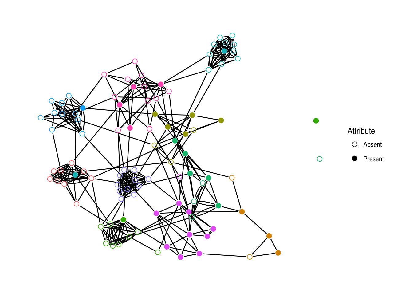
Figure 4.1: A simulated network with 100 vertices, colored according to neighborhood. The vertex fill indicates the presence or absence of the simulated attribute.
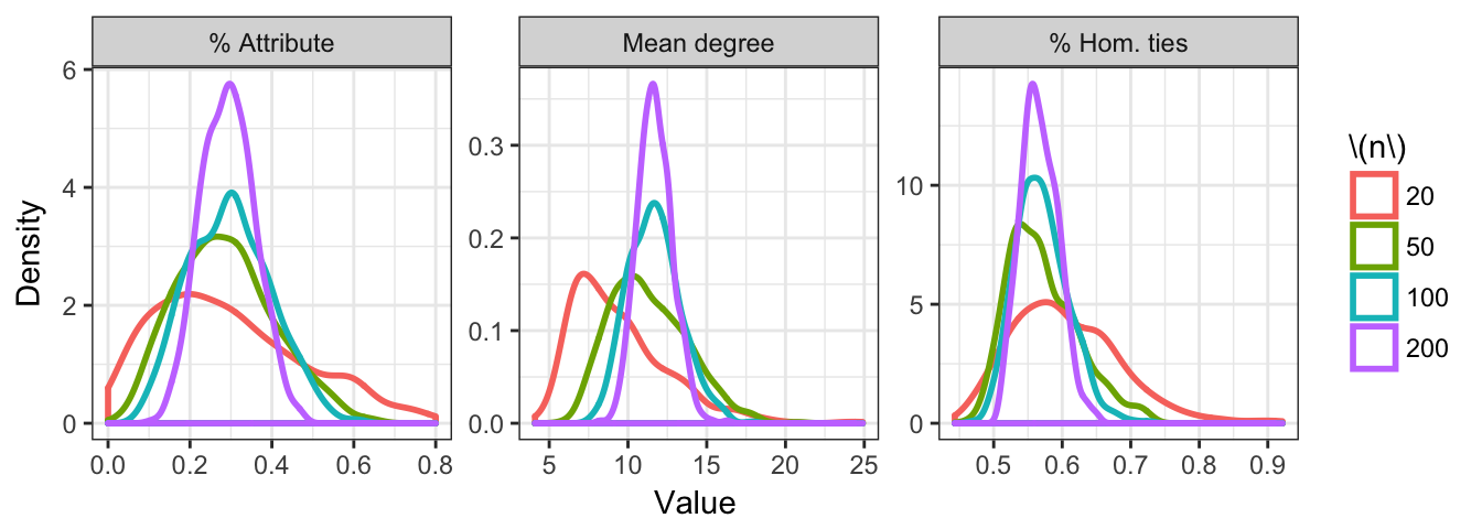
Figure 4.2: Density plots of simulated statistics of locally dependent random networks.
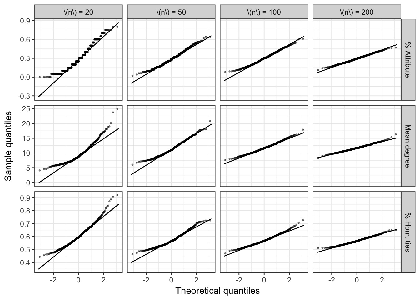
Figure 4.3: Normal Q-Q plots for simulated statistics of locally dependent random networks.
4.2 Standard error estimation
Given the asymptotic normality, all that remains to make these theorems useful for inference is to find a method to estimate the standard error of a statistic from a single observation. To that end, here we simulate a single network with 200 vertices by the same procedure as above and attempt to recover the standard errors of the statistics. We can compare these estimates to the standard errors of the empirical distributions we found in our previous simulation.
There are several approaches to approximating the standard errors. The first is to follow the vertex-level jackknife procedure outlined by Snijders & Borgatti (1999). This method is a modification of the standard jackknife estimator of standard deviation. At each iteration of the procedure, we remove one vertex from the network and recalculate the statistics of interest. Then we estimate the standard error with the equation \[\begin{equation} \widehat{\text{s.e.}} = \sqrt{\frac{n - 2}{2n} \sum_{i = 1}^{n} (g_{-i} - \bar{g})^2}, \end{equation}\]where \(g\) is the quantity whose standard error we are approximating and \(g_{-i}\) is \(g\) calculated with vertex \(i\) removed. This differs from the standard jackknife estimator in the multiplicative constant. Heuristically, this constant accounts for the fact that we are seeing much less variation in the jackknife networks than we would expect to see in the true distribution. This follows from the fact that the variance of a statistic of the edge variables is (approximately) inversely proportional to the number of edge variables, \(n(n-1)\), not the number of vertices, \(n\) (Snijders & Borgatti, 1999). We can see in Table 4.1 that this procedure underestimates the variance of our statistics.
| Statistic | Simulated standard error | Jackknife standard error |
|---|---|---|
| % Attribute | 0.0647304 | 0.0242058 |
| Mean degree | 1.1011253 | 0.8231390 |
| % Hom. ties | 0.0271141 | 0.0185213 |
| Statistic | Simulated standard error | Jackknife standard error |
|---|---|---|
| % Attribute | 0.0647304 | 0.0687571 |
| Mean degree | 1.1011253 | 1.6604948 |
| % Hom. ties | 0.0271141 | 0.0249828 |
This is most likely because of the dependence between vertices in the process that generated the network.
The second method is a standard jackknife, but leverages the neighborhood structure and the local dependence of the network. We do this by applying the jackknife at the level of the neighborhoods. That is to say, we remove each neighborhood in turn and recompute the statistic and then compute the jackknife estimator \[\begin{equation} \widehat{\text{s.e.}} = \sqrt{\frac{m-1}{m} \sum_{i = 1}^m (g_{-i} - \bar{g})^2}, \end{equation}\]where \(m\) is the number of neighborhoods. This process gives much more appropriate estimates, shown in Table 4.2.
4.3 Discussion of future work
Further development of locally dependent ERNMs for modelling complex social processes will have major impacts in the social sciences. The most pressing issue is the creation of software that allows for estimating parameters in these models. Code for fitting locally dependent ERGMs was developed by Schweinberger & Handcock (2015) and a Markov chain Monte Carlo algorithm for ERNMs was implemented by Fellows & Handcock (2012). However, it still remains to combine these two developments to work with locally dependent ERNMs.
Further mathematical work is also required to extend Theorem 3.9 to statistics involving more than one vertex attribute. This proof requires a multivariate analogue of the central limit theorem for \(M\)-dependent random variables. As my adviser told me, where there is a univariate central limit theorem, there is invariably a corresponding multidimensional theorem. However, we are unable to find a proof of this, so that result must be the topic of future work.
Finally, an investigation into the properties of standard error estimates like those produced above is much needed. Network sample sizes tend to be relatively small, so being forced to aggregate at the neighborhood level is a nontrivial issue. Furthermore, the jackknife procedure is most likely not making full use of all the information available within the observed network. However, a bootstrap procedure is, as far as my research shows, undefined for network data. Difficulty comes from being unable to sample with replacement. If one were to sample a network’s vertices or edges with replacement, most likely duplicate edges would appear in the resampled networks. It is unclear how duplicates should be handled when calculating network statistics, so that sort of procedure is difficult to define.
References
Fellows, I., & Handcock, M. S. (2012). Exponential-family random network models. ArXiv Preprint ArXiv:1208.0121.
Snijders, T. A. B., & Borgatti, S. P. (1999). Non-parametric standard errors and tests for network statistics. Connections, 22(2), 61–70.
Schweinberger, M., & Handcock, M. S. (2015). Local dependence in random graph models: Characterization, properties and statistical inference. Journal of the Royal Statistical Society: Series B (Statistical Methodology), 77(3), 647–676.