Chapter 3 Locally dependent exponential random network models

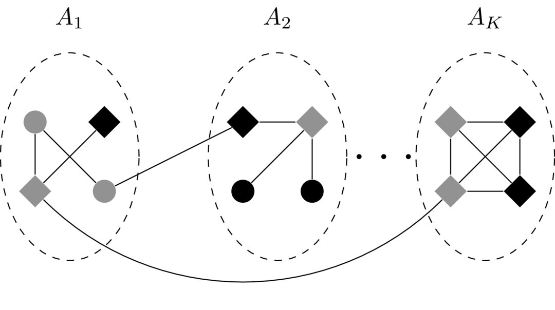
Figure 3.1: A locally dependent random network with neighborhoods A1,A2,…,AK and two binary node attributes, represented as gray or black and circle or diamond.

To begin, we define a random network, developed by Fellows & Handcock (2012). By way of motivation, note that in the ERGM the nodal variates are fixed and are included in the model as explanatory variables in making inferences about network structure. Furthermore, there is a class of models that we do not discuss here that consider the network as a fixed explanatory variable in modeling (random) nodal attributes. It is not difficult to come up with situations where a researcher would like to jointly model both the network and the node attributes. Thus we define a class of networks in which both the network structure and the attributes of the individual nodes are modeled as random quantities.

Definition 3.1 (Random network) Let N be a countable collection of nodes (which we take to be a subset of N). Let Y be the random graph on the nodes N with support Y. Then for each element n∈N, let there be a corresponding random vector of node attributes Xn∈Rq and collect them into the n×q random matrix X with support X. The is the random variable Z=(Y,X) with support Z=Y×X.

Now we wish to model these objects, so we follow the ERGM and turn to the exponential family (Fellows & Handcock, 2012). We write P(Y=y,X=x|η)∝eη⋅g(y,x). This looks very similar to the ERGM, but note the explicit dependence on the quantity x. More concretely, we can include terms that depend only on x, which would have no place in an ERGM. We can further express the difference of the two models by rewriting the left hand side of as P(X=x,Y=y|η)=P(Y=y|X=x,η)P(X=x|η), where the first term on the right hand side is the ERGM and the second term is P(X=x|η)=C(Z,η,x)C(Z,η), where C(Z,η,x)=∫{(v,u)∈Z:u=x}P(X=x|η).

Roughly, this is the proportion of the total sample space Z that is possible with x fixed. This is not, in general, equal to one, so the ERNM is not equal to the ERGM (Fellows & Handcock, 2012).

3.1 Definitions and notation

We will consistently refer to a set of nodes, Ak, as the k-th neighborhood, with an uppercase K representing the total number of neighborhoods and a lowercase k representing a specific neighborhood. The variable N will refer to the domain of a random network, usually the union of a collection of neighborhoods. Nodes within the network will be indexed by the variables i and j, with Zij=({Yij,Xi,Xj}), where Yij is referring to the edge between nodes i and j, and Xi and Xj refer to the random vectors of node attributes. Abstracting this further, i and j will also refer to tuples of nodes, so we will write →i=(i1,i2,…,iq)∈N×N×⋯×N. The variables Z and Y will also often carry a subscript of W or B (for example YBij) which emphasizes that the edge from i to j is within or between neighborhoods, respectively. Finally, for lack of a better notation, the indicator function IB(i,j) (where B is for between) is one if i∈Al and j∈Ap where l≠p, and zero otherwise.

Definition 3.2 (Local dependence property) Extending the definition in Schweinberger & Handcock (2015), a random network model satisfies if there is a partition of the node set N into neighborhoods A1,A2,…,AK for K≥2 such that the network variables Zij are dependent when i,j∈Aℓ for some ℓ and independent otherwise. We also require that nodal attributes depend only on the attributes of nodes within the same neighborhood. Thus, the probability measure can be written as P(Z∈Z)=K∏k=1[Pkk(Zkk∈Zkk)k−1∏ℓ=1Pkl(Zkl∈Zkl,Zlk∈Zlk)], where Zmn is the subnetwork consisting of the random graph ties from nodes in Am to those in An and the appropriate node variables and Zmn is a subset of the sample space of Zmn. Furthermore, the measures Pkk can induce dependence between dyads while the measures Pkl induce independence.

Definition 3.3 (Sparsity) Also from Schweinberger & Handcock (2015), we say a locally dependent random network is if there is some δ>0 and some C>0 such that E(|YBij|p)≤Cn−δ,(p=1,2) where n=|N| and YBij signifies the tie between neighborhoods from node i∈Al to node j∈Am where l≠m.

3.2 Preliminary theorems

In proving our theorems, we will make use of several other central limit theorems, all of which can be found in Billingsley (1995). The first is the Lindeberg-Feller central limit theorem for triangular arrays. The second is Lyapounov’s condition, which gives a convenient way to show that the Lindeberg-Feller theorem holds. Finally, we make use of a central limit theorem for dependent random variables. For the sake of brevity, in this section we state each of these without proof.

Theorem 3.1 (Billingsley, 1995 Theorem 27.2) For each n take Xn1,…,Xnrn, independent with E(Xns)=0 for all n and s (where no generality is lost in this assumption). Then we have σ2ns=Var(Xns)=E(X2ns). Next, set s2s=∑rns=1σ2ns. Now set Sn=Xn1+⋯+Xnrn. If the , limn→∞rn∑s=11s2n∫|Xns≥ϵsnX2ns=0 holds for all ϵ>0, then Snd→N(0,1).

Theorem 3.2 (Billingsley, 1995 Theorem 27.3) Let Sn be as before. Then if , limn→∞rn∑s=11s2+δnE(|Xns|s+δ)=0 holds for some δ>0, then the Lindeberg condition also holds. Therefore Snd→N(0,1).

Theorem 3.3 (Billingsley, 1995 Theorem 27.4) Suppose that X1,X2,… is stationary and α-mixing with αn=O(n−5) and that E(Xn)=0 and E(X12n)<∞. Note that the condition on α is stronger than what we require. Our Xn will be M-dependent, meaning that each Xn is independent of all Xm where |n−m|>M. It is true that an M-dependent sequence is α-mixing for constant α. Then, if Sn=X1+…Xn, we have Var(Sn)n→σ2. Then, if σ>0, we have Snd→N(0,1).

The final theorem is Slutsky’s theorem, a classic result of asymptotic theory in statistics.

Theorem 3.4 (Wasserman, 2004 Theorem 5.5) Let Xn,X,Yn be random variables and let c be a constant. Then, if Xnd→X and Yp→c we have Xn+Ynd→X+c and XnYnd→cX.

3.3 Consistency under sampling

With these in place, we attempt to extend a result about locally dependent ERGMs proven by Schweinberger & Handcock (2015) to locally dependent ERNMs. In short, this theorem states that the parameters estimated by modeling a small sample of a larger network can be generalized to the overall network. It was shown by Shalizi & Rinaldo (2013) that most useful formulations of ERGMs do not form projective exponential families in the sense that the distribution of a subgraph cannot be, in general, recovered by marginalizing the distribution of a larger graph with respect to the edge variables not included in the smaller graph. Hence, we are unable to generalize parameter estimates from the subnetwork to the total network.

To show that locally dependent ERNMs do form a projective family, let A be a collection of sets A, where each A is a finite collection of neighborhoods. Also, allow the set A to be an ideal, so that if A∈A, every subset of A is also in A and if B∈A, then A∪B∈A. If A⊂B, think of passing from the set A to the set B as taking a larger sample of the (possibly infinite) set of neighborhoods in the larger network. Then let {PA,θ}A∈A be the collection of ERNMs with parameter θ indexed by the sets in A. For each A∈A, let PA,Θ={PA,θ}θ∈Θ be the collection of ERNMs on the neighborhoods in A with parameter θ∈Θ where Θ⊂Rp is open. Assume that each distribution in PA,Θ has the same support ZA and that A⊂B if and only if ZB=ZA×ZB∖A. Then, the exponential family {PA,Θ}A∈A is projective in the sense of Shalizi & Rinaldo (2013 Definition 1) precisely when Theorem 3.6 holds.

This follows from a specific case of the general definition given by Shalizi & Rinaldo (2013). There, for every pair A and B with A⊂B, they define the natural projection mapping πB→A:ZB→ZA. Informally, this mapping projects the set ZB down to ZA by simply removing the extra data. For example if B={A1,A2} and A={A1} as in Figure 3.1, then the mapping πB→A is shown in Figure 3.2.

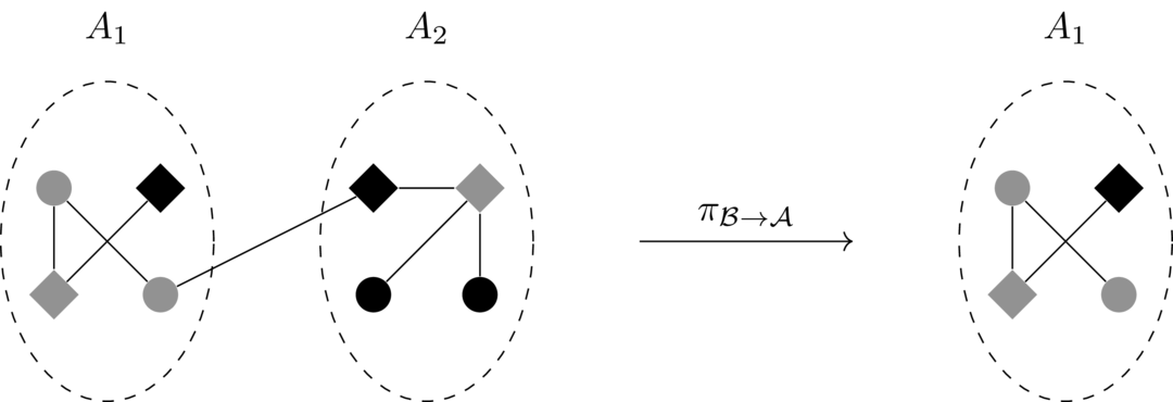
Figure 3.2: The projection mapping from B={A1,A2} to A={A1}.

This is desirable because Shalizi & Rinaldo (2013) have demonstrated the following theorem.

Theorem 3.5 (Shalizi & Rinaldo, 2013 Theorem 3) If the exponential model family {PAΘ}A∈A is projective and the log of the normalizing constant can be written as log(C(θ,Z))=log(∫Zeθ⋅g(z)dz)=r(|Z|)a(θ), where r is a positive, monotone increasing function of some positive measure on Z and a is a differentiable function of θ, then the maximum likelihood estimator exists and is strongly consistent, meaning that the MLE, ˆθa.s.→θ, where θ is the unknown parameter being estimated.

This is trivially achieved by setting r=1 for all values of |Z| and setting a(θ)=log(C(θ,Z)). We have differentiability of a with respect to θ by a result from multivariable calculus that follows from Fubini’s theorem. From a practical perspective, this means that a researcher using this model can assume that parameters estimated from samples of a large network are increasingly good approximations for the true parameter values as the sample size increases.

Theorem 3.6 Let A1,A2,… be a sequence of neighborhoods and define the sequence {NK}=⋃Ki=1Ai. Then let Z1,Z2,… be the sequence of locally dependent random networks on the NK. For each ZK, there is the corresponding set of neighborhoods AK. Let PK be a generic probability distribution from the family {PKθ}θ∈Θ. Let the network πAK+1→AK(ZK+1)=ZK+1∖K, with corresponding distirbution PK+1∖K. Then PK(ZK∈ZK)=PK+1(ZK∈ZK,ZK+1∖K∈ZK+1∖K), my_dev where ZK is the sample space of the distribution PK and ZK⊂ZK. This is a specific case of the definition of projectibility for a general exponential family given by Shalizi & Rinaldo (2013).

Proof. This follows from the definition of local dependence, in much the same way as the proof for ERGMs by Schweinberger & Handcock (2015) does. We have PK+1(ZK∈ZK,ZK+1∖K∈ZK+1∖K)=PK+1(ZK∈ZK)PK+1∖K(ZK+1∖K∈ZK+1∖K)=PK(ZK∈ZK)(1)=PK(ZK∈ZK), where the measure becomes Pk from the product definition of a locally dependent random network.

3.4 Asymptotic normality of statistics

In this section we will prove that certain classes of statistics of locally dependent random networks are asymptotically normally distributed as the number of neighborhoods tends to infinity. The statistics we consider can be classified into three types: first, statistics which depend only on the graph structure; second, statistics that depend on both the graph and the nodal variates; and third, statistics that depend only on the nodal variates. The first class of statistics has already been considered by Schweinberger & Handcock (2015), but we will reproduce the proof here, as the second proof is very similar. The third class of statistics becomes normal in the limit by a central limit theorem for M dependent random variables in Billingsley (1995).

Before we begin to explicitly define each of these classes, we clarify the notation that will be used. A general statistic will be a function S:Nd→R, where Nd is the d-fold Cartesian product of the set of nodes, N, with itself: Nd=N×⋯×N⏟d times.

Additionally, the statistic will often carry a subscript K, indicating that the statistic is of the random network with K neighborhoods.

Formally, as explained in Schweinberger & Handcock (2015), the first class of statistics contains those that have the form SK=∑i∈NdSKi, where SKi=∏l,p∈iYlp,

a product q of edge variables that captures the interaction desired. We will also make use of the set Adk, wich is a similar cartesian product. When we write i∈Adk, we mean the every component of the d-tuple i is an element of Ak. Furthermore, by a catachrestic abuse of notation, we will write l,p∈i to mean that l and p are vertices contained in the d-tuple i. Now we are ready to prove the first case of the theorem.

Theorem 3.7 Let A1,A2,…,AK be a sequence of neighborhoods of size at most M and form the sequence of domains NK=⋃Kk=1Ak. Then let Z1,Z2,…,ZK be the sequence of unweighted random networks on the NK. Then, let the statistic SK:NdK→R be given. Furthermore, assume the statistic depends only on the graph variables of the ZK. We also assume that the ZK satisfy the local dependence property and that they are δ-sparse, for some δ>d. Finally, we require that Var(W∗K)→∞, where W∗K is defined in (3.3). Then SK−E(SK)√Var(SK)d→K→∞N(0,1).

Proof. As the networks ZK are unweighted, all edge variables Yij∈{0,1}. Let μij=E(Yij). Then define Vij=Yij−μij. Therefore, without loss of generality, we may work with Vij, which has the convenient property that E(Vij)=0. This means that we can similarly shift our statistics of interest, SK. Therefore, call S∗K=SK−E(SK), so that E(S∗K)=0.

Note that we can write S∗K=W∗K+B∗K, with W∗K=K∑k=1W∗K,k=K∑k=1∑i∈NdKI(i∈Adk)S∗Ki and B∗K=∑i∈NdKIB(i)S∗Ki,

where the indicator functions restrict the sums to within the k-th neighborhood and between neighborhoods of the graph, respectively. Specifically, IB(i)=1 when the d-tuple of nodes i contains nodes from different neighborhoods, or exactly when I(i inAdk)=0 for all neighborhoods k. By splitting the statistic into the within and between neighborhood portions, we are able to make use of the independence relation between edges that connect neighborhoods. We also have E(W∗K)=0 and E(B∗K)=0, as each quantity is a sum of random variables with mean zero.

The idea of this proof is to gain control over the variances of B∗K and all the elements of the sequence W∗Kk. We can then show that B∗K is converging in probability to zero and that the triangular array W∗K satisifies Lyaponouv’s condition, and is thus asymptotically normal. Finally, Slutsky’s theorem allows us to extend the result to S∗K.

To bound the variance of B∗K, note that Var(B∗K)=∑i∈NdK∑j∈NdKIB(i)IB(j)Cov(S∗Ki,S∗Kj). Despite independence, some of these covariances may be nonzero if the two terms of the statistic both involve the same edge. For example, in Figure , a statistic that counted the number of edges between gray nodes plus the number of edges between diamond shaped nodes would have a nonzero covariance term because of the edge between the two nodes that are both gray and diamond shaped. To show that, in the limit, these covariances vanish, we need only concern ourselves with the nonzero terms in the sum. That is, only those terms where IB(i)IB(j)=1. This happens exactly when both S∗Ki and S∗Kj involve a between neighborhood edge variable. So, note that we have Cov(S∗Ki,S∗Kj)=E(S∗KiS∗Kj)−E(S∗Ki)E(S∗Kj)=E(S∗KiS∗Kj), as the expectation of each term is zero. Next we take Yl1l2 to be one of the (possibly many) between neighborhood edge variables in this product (such that IB(i)=1 where i is any tuple containing l1 and l2) and Vl1l2 to be the recentered random variable corresponding to Yl1l2. Then, Cov(S∗Ki,S∗Kj)=E(∏m,n∈iVmn∏m,n∈jVmn)=E(Vpl1l2∏m,n∈(i∪j)∖{l1,l2}Vmn),(p=1,2) where we must consider the case where p=1 to account for the covariance of S∗Ki and S∗Kj when i≠j and the case where p=2 to account for the variance of S∗Ki, which is computed in the case where i=j. So, if p=1, then E(Vl1l2∏m,n∈(i∪j)∖{l1,l2}Vmn)=E(Vl1l2)E(∏m,n∈(i∪j)∖{l1,l2}Vmn)=0, by the local dependence property and the assumption that E(Vl1l2)=0. The local dependence property allows us to factor out the expectation of Vl1l2, as this edge is between neighborhoods, and therefore independent of every other edge in the graph. Now, if we have p=2, then, by sparsity and the fact that the product below is at most 1, E(V2l1l2)E(∏m,n∈(i∪j)∖{l1,l2}Vmn)≤DCn−δ, where D is a constant that bounds the expectation above. There exists such a constant because each of the V_{mn} are bounded by definiton, so a product of them is bounded. So as K grows large, the between neighborhod covariances all become asymptotically negligible. Therefore, we can conclude that Var(B∗K)=∑i∈NdK∑j∈NdKIB(i)IB(j)Cov(S∗Ki,S∗Kj)≤DCn2d(−δ). So we have VarB∗K→0. Then, for all ϵ>0, Chebyshev’s inequality gives us limK→∞P(|B∗K|>ϵ)≤limK→∞1ϵ2Var(B∗K)=0, so B∗Kp→K→∞0. Next, we bound the within neighborhood covariances, as we also have Var(W∗Kk)=∑i∈NdK∑j∈NdKI(i,j∈Ak)Cov(S∗Ki,S∗Kj). As the covariance forms an inner product on the space of square integrable random variables, the Cauchy-Schwarz inequality gives us I(i,j∈Ak)|Cov(S∗Ki,S∗Kj)|≤I(i,j∈Ak)√Var(S∗Ki)√Var(S∗Kj). Then, as each S∗Ki has expectation zero, we know that Var(S∗Ki)=E(S∗2Ki)−E(S∗Ki)2=E(S∗2Ki). As S∗2Ki≤1, we know Var(S∗Ki)≤1 for all tuples i, so we have the bound I(i,j∈Ak)|Cov(S∗Ki,S∗Kj)|≤I(i,j∈Ak). Now all that remains is to apply the Lindeberg-Feller central limit theorem to the double sequence W∗K=∑Kk=1W∗K,k. To that end, first note that, as each neighborhood contains at most a finite number of nodes, M, we can show that Var(W∗K,k)=∑i∈NdK∑j∈NdKI(i,j∈Adk)Cov(S∗Ki,S∗Kj)=∑i∈NdK∑j∈NdKI(i,j∈Adk)E(S∗KiS∗Kj)≤∑i∈NdK∑j∈NdK1≤M2d. Now we prove that Lyaponouv’s condition (3.2) holds for the constant in the exponent δ=2. So limK→∞K∑k=11Var(W∗K)2E(|W∗K,k|4)=limK→∞1Var(W∗K)2K∑k=1E(W∗2K,k)E(W∗2K,k)≤limK→∞M2dVar(W∗K)2K∑k=1E(W∗K,k)2=limK→∞M2dVar(W∗K)2K∑k=1Var(W∗K,k)=limK→∞M2dVar(W∗K)=0. where Var(W∗K) tends to infinity by assumption. Therefore, Lyaponouv’s condition holds, and so by the Lindeberg-Feller central limit theorem, we have, W∗K√Var(W∗K)d→K→∞N(0,1). Slutsky’s theorem (3.4) gives the final result for S∗K=W∗K+B∗K. Then we have S∗K√Var(S∗K)d→K→∞N(0,1), as desired.

The second class of statistics are those that depend on both the graph and the nodal variates. These have a very similar form as the statistics previously considered. Now we require that SK=∑i∈NdSKi, where SKi=∏l,p∈iYlph(Xl,Xp),

a product with at most q terms.

Theorem 3.8 If SK is a statistic depending on both the random graph and the random nodal attributes, the sequence of random networks are as before, and the function h is uniformly bounded in the sense that, for all l and m, there is some B such that P(|h(Xl,Xm)|p>B)=0,(p=1,2) then we also have SKd→K→∞N(0,1).

Proof. This proof is very similar to the proof of Theorem 3.7. We write SK=WK+BK,

exactly as before, incorporating the function h into each SKi as we did above. Then the binary nature of the graph and the uniform boundedness of h allow us to once again recenter the Yij, meaning that we will work with Vijh(Xi,Xj)=Yijh(Xi,Xj)−μij. We also have E(Vijh(Xi,Xj))=0, so E(S∗Ki)=0 as well.

For the between neighborhood covariances, we once again choose Vl1l2, a between neighborhood network variable. Then we once again write Cov(S∗Ki,S∗Kj)=E(∏m,n∈iVmnh(Xm,Xn)∏m,n∈jVmnh(Xm,Xn))=E((Vl1l2h(Xl1,Xl2))p∏m,n∈(i∪j)∖{l1,l2}Vmnh(Xm,Xn)),(p=1,2)=E((Vl1l2h(Xl1,Xl2))p)E(∏m,n∈(i∪j)∖{l1,l2}Vmnh(Xm,Xn)), by the local dependence property. Then, when p=1, we have E(Vl1l2h(Xl1,Xl2))=0 by assumption, so the covariance is identically zero. When p=2 we have E((Vl1l2h(Xl1,Xl2))2)≤Cn−δ by sparsity and E(∏m,n∈(i∪j)∖{l1,l2}Vmnh(Xm,Xn))≤(DB)2q−2 almost surely by uniform boundedness and the fact this product has at most 2q−2 terms. This follows from the fact that h is bounded by B and that Vmn is bounded by some constant D, by defintion. So Cov(S∗Ki,S∗Kj)≤B2q−2Cn−δ, which tends to zero as K grows large. So, again by Chebyshev’s inequality, we have B∗Kp→K→∞0. Next we bound the within neighborhood covariances. Now with each |S∗Ki|≤Bq, we have I(i,j∈Ak)|Cov(S∗Ki,S∗Kj)|≤I(i,j∈Ak)B2q. Now, we show that Lyaponouv’s condition (3.2) holds for the same δ=2. Once again note that each neighborhood has at most M nodes, so Var(W∗K,k)=∑i∈NdK∑j∈NdKI(i,j∈Ak)Cov(S∗Ki,S∗Kj)≤∑i∈NdK∑j∈NdKI(i,j∈Ak)B2q≤M2dB2q. Then Lyaponouv’s condition is limK→∞K∑k=11Var(W∗K)2E(|W∗K,k|4)=limK→∞1Var(W∗K)2K∑k=1E(W∗2K,k)E(W∗2K,k)≤limK→∞M2dB2qVar(W∗K)2K∑k=1E(W∗2K,k)=limK→∞M2dB2qVar(W∗K)2K∑k=1Var(W∗K,k)=limK→∞M2dB2qVar(W∗K)=0. Therefore, by the Lindeberg-Feller central limit theorem and Slutsky’s theorem, we have S∗K√Var(S∗K)d→K→∞N(0,1).\qedhere

Finally, the last class of statistic is that which depends only on the nodal variates. This result follows directly from a central limit theorem for M-dependent random variables, which can be found in Billingsley (1995, p. 364). Establishing this theorem requires that we assume that the statistic in question depends only on a single variable across nodes. Therefore we assume that the statistic depends only on a single nodal covariate.

Theorem 3.9 Take the sequence ZK as before, and let XK be the vector of nodal variates for each ZK. Call each entry of this vector XKi, the variate corresponding to node i. Furthermore, we assume that E(X12Ki)<∞, E(XKi=0). Then, limK→∞Var(∑ni=1XKi)n=σ2, where n=|N|. Furthermore, if σ>0, then ∑ni=1XKi√nVar(∑ni=1XKi)d→K→∞N(0,1).

Proof. Two random variables XKl and XKp are dependent if and only if l and p are in the same neighborhood. Without loss of generality, assume that the neighborhoods are such that all nodes within a neighborhood are indexed by consecutive integers. Then let M=lim sup|AK|. Then the sequence XKl is M-dependent, so the result follows by application of Theorem 27.4 in Billingsley (1995).

In practice, the hypothesis that the twelfth moment exists is satisfied for most reasonable distributional assumptions about nodal covariates. Furthermore, the assumption that all nodal variates have expectation zero can easily be satisfied by recentering the observed data. Finally, the delta method gives us an asymptotically normal distribution for a differentiable statistic of the nodal variate. The univariate nature of the statistic is a fundamental limitation of this approach, however I am unable to find an analogous multidimensional central limit theorem that would allow us to establish the asymptotic normality of a statistic of multiple nodal variates.

References

Fellows, I., & Handcock, M. S. (2012). Exponential-family random network models. ArXiv Preprint ArXiv:1208.0121.

Schweinberger, M., & Handcock, M. S. (2015). Local dependence in random graph models: Characterization, properties and statistical inference. Journal of the Royal Statistical Society: Series B (Statistical Methodology), 77(3), 647–676.

Billingsley, P. (1995). Probability and measure (3. ed., authorized reprint). New Delhi: Wiley India.

Shalizi, C. R., & Rinaldo, A. (2013). Consistency under sampling of exponential random graph models. The Annals of Statistics, 41(2), 508–535. http://doi.org/10.1214/12-AOS1044