Chapter 2 Exponential random graph models
The first model of interest to this thesis is the exponential random graph model (ERGM), introduced by S. Wasserman & Pattison (1996). Broadly, given a network, this model allows us to specify structural features that are of interest and test in a principled way if there are more of those kinds of features present than would be expected if the network were formed by chance. This allows the researcher to draw conclusions about the latent process that generated the network.
This model can be expressed by the equation \[\begin{equation} P(Y = y | \theta) = \frac{e^{\theta \cdot g(y)}}{C(\theta, \mathcal{Y})} \tag{2.1}, \end{equation}\]where \(g(y)\) is a vector of statistics that depend on the network \(y\) and \(\theta\) is a vector of parameters. The function \(C(\theta, \mathcal{Y})\) is a normalizing constant. We may easily extend the model to include nodal covariates (like demographic information) by introducing the fixed \(n \times p\) matrix \(x\) which is used to calculate some of the components of \(g\).
Note that the constant in the denominator depends both on the support of the random variable \(Y\), which is fixed and—in principle—known, and the unknown parameter \(\theta\). In general, this constant will have the form \[\begin{equation} C(\theta, \mathcal{Y}) = \sum_{y \in \mathcal{Y}} e^{\theta \cdot g(y)}, \tag{2.2} \end{equation}\]which is impossible to compute in all but the most trivial cases, as the sum is over all possible networks. For the simplest undirected binary network with \(n\) nodes, we have \(\left| \mathcal{Y} \right| = 2^{n(n-1)/2},\) so for 10 nodes, the constant \(C\) will be a sum of \(2^{45}\) terms. As each term requires a non-trivial calculation, we are unable to calculate the value of \(C\) directly for a network of any reasonable size.
With the model in place, we can begin to estimate the parameter \(\theta\) via maximum likelihood estimation. To do that, we define the likelihood function, which takes the parameter space into the reals. Our goal is to find the value of \(\theta\) that maximizes this function given the observed data. We call this \(\theta\) the maximum likelihood estimator, or MLE. Intuitively, we are looking for the value of \(\theta\) that makes the network we have observed most likely according to our model. In our case this function is \[\begin{equation} L(\theta | y) = \frac{e^{\theta \cdot g(y)}}{C(\theta, \mathcal{Y})}. \tag{2.3} \end{equation}\]Note that \(C\) also varies with \(\theta\).
The fact that this term varies with \(\theta\) means that a naive optimization algorithm will be prohibitively slow. Exploring the parameter space almost always involves evaluating the function at many different points. For example, the common gradient descent algorithm involves evaluating the function many times in the neighborhood of a point to approximate the gradient. This then allows the algorithm to choose a new point where the function is larger. This process then repeats. Even when given relatively simple functions, this algorithm can require hundreds of function calls. In our case, that is not feasible, as we cannot even evaluate our function once.
2.1 Finding parameter estimates
The intractable normalizing constant (2.2) makes fitting this model directly extremely difficult. With no general analytic method to maximize the likelihood, we must turn to numerical approximations. However, these algorithms involve evaluating \(L(\theta)\) at many different points. When \(\theta\) varies the value of \(C\) also changes, so each function evaluation must recompute this enormous sum. This makes standard numerical approaches useless for the problem at hand. Despite this there are several approaches that make use of a variety of approximations to (we hope) find reasonable parameter estimates. Here we will present both frequentist and Bayesian methods for estimating \(\theta\). To begin, we introduce another piece of notation.as desired.
Thus, each component of \(\theta\) represents the increase in the log-odds of a tie from \(i\) to \(j\) being present in the network that is associated with a change in \(y^{c}_{ij}\) that increases the corresponding component of \(g(y)\) by one unit. An example of this kind of interpretation is presented in Section 2.2.
2.1.1 Frequentist methods
The change statistic allows us to define the pseudolikelihood, introduced by Strauss & Ikeda (1990). The pseudolikelihood function represents the model where the probability that a tie from \(i\) to \(j\) exists is independent of all the other ties. Even when this assumption is known to be false, the hope is that the maximum pseudolikelihood estimator will be a good approximation of the more general MLE. This yields the likelihood function \[\begin{equation*} \operatorname{PL}(\theta) = \prod_{i \neq j}P(Y_{ij} = y_{ij} | \theta). \end{equation*}\]Taking the logit transforms this into a standard logistic regression where the response variable is the vector containing a 1 or a 0 depending on the existence of the tie between nodes \(i\) and \(j\) and the explanatory variables are the vectors of change statistics. This can then easily be fit using widely available generalized linear modeling tools. The estimator returned by this logistic regression is called the maximum psuedolikelihood estimator (MPLE).
However, this method exhibits a few problems. In many cases, as already discussed, the assumption of dyadic independence is not justifiable, so the coefficient estimates cannot be expected to be accurate in general. The class of models called dyadic independence models are those in which the form of \(g\) makes the likelihood exactly equal to the psuedolikelihood, and so we can fit them exactly using this method. When the dyadic independence assumption does not hold, we are no longer maximizing the likelihood associated with our model, so there is no reason to expect that we have the properties that make maximum likelihood estimators so nice. Specifically, there is no reason to believe that the parameter estimates actually asymptotically approach the true values or that the estimates are approximately normally distributed with the reported standard errors. An example of the trouble with standard errors will be seen in Section 2.2.
It is clear that a better method for computing the maximum likelihood estimator is highly desirable. This brings us to the Markov chain Monte Carlo MLE (MCMC-MLE) algorithm developed by Geyer & Thompson (1992). They introduce a method with applications to intractable distributions beyond ERGMs, but we will remain within that specific context. The crux of the algorithm lies in choosing a fixed value \(\theta_0\) (typically the MPLE) that we hope is close to the true value of \(\theta\) and then maximizing the likelihood ratio \[\begin{equation} \log \left[\frac{L(\theta)}{L(\theta_0)} \right]. \tag{2.5} \end{equation}\] We begin with the log likelihood of model (2.1) \[\begin{equation} \ell(\theta) = \theta \cdot g(y) - \operatorname{log} \left( C(\theta, \mathcal{Y}) \right). \tag{2.6} \end{equation}\] We can rewrite the ratio (2.5) as \[\begin{equation} \ell(\theta) - \ell(\theta_{0}) = (\theta - \theta_{0}) \cdot g(y) - \operatorname{log} \left( \frac{C(\theta, \mathcal{Y})}{C(\theta_{0}, \mathcal{Y})} \right). \tag{2.7} \end{equation}\] Clearly, this is maximized at the same value of \(\theta\) as the original likelihood, but now we can show that \[\begin{equation} \frac{C(\theta, \mathcal{Y})}{C(\theta_{0}, \mathcal{Y})} = \mathbb{E}_{\theta_0} \left[ e^{(\theta - \theta_0) \cdot g(y)} \right]. \tag{2.8} \end{equation}\] This follows from noting that \[\begin{align*} \frac{C(\theta, \mathcal{Y})}{C(\theta_{0}, \mathcal{Y})} &= \frac{\sum_{z \in \mathcal{Y}} e^{\theta \cdot g(z)}}{\sum_{w \in \mathcal{Y}} e^{\theta_{0} \cdot g(w)}} \\ &= \frac{\sum_{z \in \mathcal{Y}} e^{\theta \cdot g(z)} e^{(\theta_0 - \theta_0) \cdot g(z)}}{\sum_{w \in \mathcal{Y}} e^{\theta_{0} \cdot g(w)}} \\ &= \sum_{z \in \mathcal{Y}} \left[ e^{\theta \cdot g(z)} e^{-\theta_0 \cdot g(z)} \left( \frac{e^{\theta_0 \cdot g(z)}}{\sum_{w \in \mathcal{Y}} e^{\theta_0 \cdot g(w)}} \right) \right]. \end{align*}\]Recognizing the term in parentheses as \(P_{\theta_0} (Y = z)\) makes it clear that we have \[ \frac{C(\theta, \mathcal{Y})}{C(\theta_{0}, \mathcal{Y})} = \sum_{z \in \mathcal{Y}} e^{(\theta - \theta_0) \cdot g(z)} P_{\theta_0} (Y = z) = \mathbb{E}_{\theta_0}\left[ e^{(\theta - \theta_{0}) \cdot g(Y)} \right], \] as desired. Now we need only estimate this expectation using the weak law of large numbers. We do this by generating a Markov chain with stationary distribution \(P_{\theta_0}\) and sampling sufficiently many times to get a good approximation of (2.8).
Hence, the problem is reduced to constructing a Markov chain with \(P_{\theta_0}\) as its stationary distribution. We use the algorithm developed by Morris, Handcock, & Hunter (2008). It is essentially a Metropolis-Hastings algorithm where the proposal distribution chooses a pair of nodes, also called a dyad, then if they are connected, removes that tie, and if they are not connected, adds a tie between them. The obvious proposal distribution chooses two vertices at random, producing a simple random walk on \(\mathcal{Y}\). As an alternative to this naïve proposal distribution, Morris et al. (2008) and M. S. Handcock et al. (2016) have developed the tie-no-tie, or TNT, proposal distribution. In this method, the dyad is chosen by first selecting whether we will toggle a dyad with or without a tie in the original network. Then a pair of nodes from within the set of those which are either connected or not connected (depending on the previous step) is chosen at random. According to its inventors, this modification of the random walk on \(\mathcal{Y}\) causes the chain to mix better, especially in sparse networks.
This allows us to approximate samples from the probability distribution on \(\mathcal{Y}\) implied by the parameter \(\theta_0\). Then we can estimate the expected value in (2.8) and calculate what we hope is a good estimate for the actual MLE. However, this method is not without its caveats. It is shown in Hunter, Handcock, Butts, Goodreau, & Morris (2008) that this algorithm can be sensitive to the initial parameter \(\theta_0\) and a poor choice of this parameter can cause the approximation of the likelihood function (2.7) to never achieve a maximum on the parameter space. This happens when the function that we are optimizing, an approximation of the true log likelihood ratio, is bad enough that it becomes unbounded and so numeric optimization routines fail to find the maximum.
2.1.2 Bayesian methods
The parameter \(\theta\) may also be estimated by Bayesian methods. However, this introduces the issue of sampling from a “doubly intractable” posterior distribution, where the problem of incalculable normalizing constants in the posterior is compounded by the functional form of our model (2.1). Markov chain Monte Carlo methods for these distributions have been studied by Murray, Ghahramani, & MacKay (2012), where the easy to implement exchange algorithm was introduced, and Caimo & Friel (2011), where this algorithm was applied to ERGMs. The algorithm very cleverly avoids the intractable constants in (2.1) by augmenting the posterior with an auxiliary variable from the same sample space as the parameter of interest. By doing this in just the right way, we are able to cancel all intractable constants from the acceptance probability (2.10).
To be precise, let the observed network \(y\) be taken from the distribution \(P_{\theta}\) and let the prior for \(\theta\) have distribution \(p(\theta)\). We must construct a Markov chain with stationary distribution equal to the posterior given by \[\begin{equation} \pi(\theta | y) = \frac{P_{\theta}(Y = y) p(\theta)}{\int P_{\theta}(Y = y) p(\theta) \; \mathrm{d}\theta}. \tag{2.9} \end{equation}\] In a standard Metropolis-Hastings implementation with proposal distribution =\(\theta^{\prime} \sim q( \cdot | \theta)\) =500 we would have the acceptance probability \[\begin{equation} a = \min \left[ 1, \frac{P_{\theta^{\prime}}(Y = y)p(\theta^{\prime})q(\theta^{\prime}|\theta)}{P_{\theta}(Y = y)p(\theta)q(\theta|\theta^{\prime})} \right], \tag{2.10} \end{equation}\] where the likelihoods in the numerator and the denominator are evaluated at different values of \(\theta\). For the ERGM, the normalizing constants will not cancel. To get around this, we take \(w \sim P_{\theta^{\prime}}\) and \(\theta^{\prime} \sim q(\cdot|\theta)\). Here, \(w\) is another network that we sample from the ERGM distribution with parameter \(\theta^{\prime}\), while \(\theta^{\prime}\) is drawn from an arbitrary proposal distribution that can depend on the current value of \(\theta\). Now the distribution we are sampling from is \[\begin{equation} \pi(\theta, \theta^{\prime}, w |y) = \frac{P_{\theta}(Y = y) P_{\theta^{\prime}}(Y = w) q(\theta^{\prime} | \theta) p(\theta)}{\int P_{\theta}(Y = y) P_{\theta^{\prime}}(Y = w) q(\theta^{\prime} | \theta) p(\theta) \; \mathrm{d} \theta}. \tag{2.11} \end{equation}\] The conditional distribution of \(\theta\) is the posterior we are after. To begin, we draw \(\theta^{\prime}\) from the (arbitrary) distribution \(q\), which can depend on \(\theta\). Then we draw \(w\) from the distribution implied by \(\theta^{\prime}\) (using already developed MCMC routines) and we propose an exchange of the generated data \(w\) and the observed data \(y\) between the parameters \(\theta\) and \(\theta^{\prime}\) which is accepted with probability \[\begin{equation} a = \min \left[ 1, \frac{P_{\theta^{\prime}}(Y = y) P_{\theta}(Y=w)p(\theta^{\prime})q(\theta^{\prime}|\theta)}{P_{\theta}(Y = y)P_{\theta^{\prime}}(Y = w)p(\theta)q(\theta|\theta^{\prime})} \right]. \tag{2.12} \end{equation}\]Now all the incalculable constants in (2.12) cancel, and we can approximate the posterior distribution as desired.
It was also demonstrated by Caimo & Friel (2011) that in most cases the use of adaptive direction sampling (ADS) allows for a more thorough exploration of the state space in fewer iterations. This improvement involves running multiple chains (say twice as many as the number of parameters in the model) that, at each iteration \(i\), are updated separately. When updating the \(j\)-th chain, two other chains, \(k\) and \(\ell\) are randomly selected, then we propose \(\theta_{j}^{\prime} = \gamma (\theta^{i}_{k} - \theta^{i}_{\ell}) + \epsilon\) where \(\gamma\) is a fixed tuning parameter and \(\epsilon\) is a small random quantity, both chosen to achieve a higher level of mixing than is usually seen when running a single chain in isolation. This improves the overall mixing of the separate chains and allows the process to thoroughly explore the sample space in fewer iterations. This is the default method in the Bergm package.
2.2 Examples
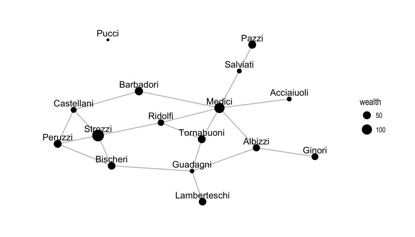
Figure 2.1: A plot of the Florentine marriage network where node size indicates wealth in thousands of lira.
ergm package by M. S. Handcock et al. (2016), which we also use to fit MPLE and MCMC-MLE models. We will use the Bergm package by Caimo & Friel (2014) to fit the Bayesian models. These data consist of an undirected network of marriages between Florentine families during the Renaissance, along with several nodal covariates, including the family wealth in thousands of lira in the year 1427. This network is drawn in Figure 2.1. We will fit the ERGM with network statistics
\[\begin{equation}
g(y) = \left( \sum_{i < j} y_{ij}, \sum_{i < j < k} y_{ij} y_{jk} y_{ki}, \sum_{i < j} y_{ij} \left| x_{i} - x_{j} \right| \right),
\tag{2.13}
\end{equation}\]
where \(y\) is the network and \(x\) is the corresponding vector of wealth measurements. Simply put, this creates a term for the number of edges, the number of triangles, and the difference in wealth between connected nodes in the network. The edge term acts as a sort of intercept in the model by measuring the overall propensity of actors to form ties, the triangle term measures the propensity of actors in the graph to form triangles, and the wealth difference term accounts for how difference in family fortune affects the probability of tie formation. Tables 2.1, 2.2, and 2.3 show the coefficient estimates and standard errors. Bayesian estimation is done using a very flat multivariate normal prior centered on the origin with variance-covariance matrix
\[\begin{equation*}
\Sigma =
\begin{bmatrix}
100 & 0 & 0 \\
0 & 100 & 0 \\
0 & 0 & 100 \\
\end{bmatrix}.
\end{equation*}\]
Figure 2.2 shows posterior density estimates for the Bayesian model.
| term | estimate | std.error |
|---|---|---|
| edges | -2.36 | 0.44 |
| triangle | 0.16 | 0.44 |
| absdiff.wealth | 0.02 | 0.01 |
| term | estimate | std.error |
|---|---|---|
| edges | -2.29 | 0.45 |
| triangle | -0.04 | 0.60 |
| absdiff.wealth | 0.02 | 0.01 |
| term | posterior mean | posterior s.d. |
|---|---|---|
| edges | -2.25 | 0.45 |
| triangle | -0.33 | 0.59 |
| absdiff.wealth | 0.02 | 0.01 |
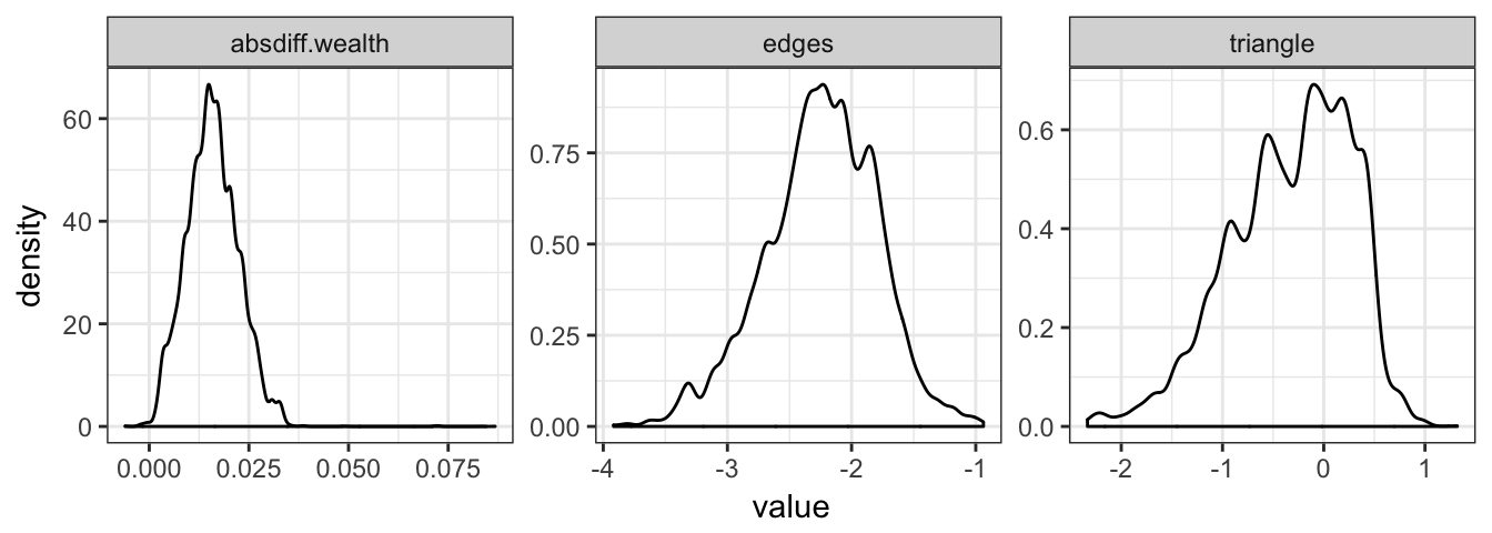
Figure 2.2: Posterior density plots of the Florentine marriage model parameter estimates.
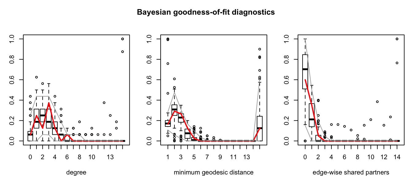
Figure 2.3: Goodness-of-fit assessment for the Bayesian model fit to the Florentine marriage data. These plots compare simulated distributions of graph statistics that were not modeled to the observed values (in red).
We can see that all of these methods produce similar outcomes, with a clearly nonzero edge term, which makes sense as this is akin to an intercept term in a standard linear model, and a small but significant term corresponding to the difference in wealth. Notice that the standard error of the triangle term (which creates dependence between dyads) is much larger when the model is fit using MCMC-MLE. This supports the notion that standard errors reported my MPLE are unreliable in dyadic dependence models, as was discussed in Section 2.1.1. Interpreting these coefficients allows us to infer that a difference in wealth of 1 unit (in this case 1000 lira), changes the log-odds of forming a tie (according to the MCMC-MLE model) by a factor of \(\theta_3 \approx\) -0.04. The ergm and Bergm packages also provide tools for assessing the goodness-of-fit of exponential random graph models. These tools simulate many networks from the distribution implied by the model with the parameter estimate and then compare the distributions of several network statistics that were not modeled to the observed network. These statistics are by default minimum geodesic distance, edgewise shared partners, and degree distribution. Figure 2.3 shows plots of these comparisons for the Bayesian model. As we can see, our model matches the simulated distributions fairly well.
References
Wasserman, S., & Pattison, P. (1996). Logit models and logistic regressions for social networks: I. an introduction to markov graphs and p*. Psychometrika, 61(3), 401–425.
Strauss, D., & Ikeda, M. (1990). Pseudolikelihood estimation for social networks. Journal of the American Statistical Association, 85(409), 204–212. Retrieved from http://www.jstor.org/stable/2289546
Geyer, Charles J., & Thompson, E. A. (1992). Constrained monte carlo maximum likelihood for dependent data. Journal of the Royal Statistical Society. Series B (Methodological), 54(3), 657–699. Retrieved from http://www.jstor.org/stable/2345852
Morris, M., Handcock, M. S., & Hunter, D. R. (2008). Specification of exponential-family random graph models: Terms and computational aspects. Journal of Statistical Software, 24(4).
Handcock, M. S., Hunter, D. R., Butts, C. T., Goodreau, S. M., Krivitsky, P. N., & Morris, M. (2016). ergm: Fit, simulate and diagnose exponential-family models for networks. The Statnet Project (http://www.statnet.org). Retrieved from http://CRAN.R-project.org/package=ergm
Hunter, D. R., Handcock, M. S., Butts, C. T., Goodreau, S. M., & Morris, M. (2008). ergm: A package to fit, simulate and diagnose exponential-family models for networks. Journal of Statistical Software, 24(3).
Murray, I., Ghahramani, Z., & MacKay, D. (2012). MCMC for doubly-intractable distributions. ArXiv Preprint ArXiv:1206.6848.
Caimo, A., & Friel, N. (2011). Bayesian inference for exponential random graph models. Social Networks, 33(1), 41–55. http://doi.org/10.1016/j.socnet.2010.09.004
Caimo, A., & Friel, N. (2014). Bergm: Bayesian exponential random graphs in R. Journal of Statistical Software, 61(2). Retrieved from http://www.jstatsoft.org/v61/i02/