In this blog post I hope to introduce you to the powerful and simple Metropolis-Hastings algorithm. This is a common algorithm for generating samples from a complicated distribution using Markov chain Monte Carlo, or MCMC.
By way of motivation, remember that Bayes’ theorem says that given a prior \(\pi(\theta)\) and a likelihood that depends on the data, \(f(\theta | x)\), we can calculate \[ \pi(\theta | x) = \frac{f(\theta | x) \pi(\theta)}{\int f(\theta | x) \pi(\theta) \; \mathrm{d}\theta}. \]
We call \(\pi(\theta | x)\) the posterior distribution. It’s this distribution that we use to make estimates and inferences about the parameter \(\theta\). Often, however, this distribution is intractable; it can’t be calculated directly. This usually happens because of a nasty integral in the denominator that isn’t easily solvable. In cases like this, the best solution is usually to approximate the posterior using a Monte Carlo method.
The algorithm
The Metropolis-Hastings algorithm is a powerful way of approximating a distribution using Markov chain Monte Carlo. All this method needs is an expression that’s proportional to the density you’re looking to sample from. This is usually just the numerator of your posterior density.
To present the algorithm, let’s start by assuming the distribution you want to sample from has density proportional to some function \(f\). You’ll also need to pick what’s called a “proposal distribution” that changes location at each iteration in the algorithm. We’ll call this \(q(x | \theta)\). Then the algorithm is:
- Choose some initial value \(\theta_0\).
- For \(i = 1, \dots, N\):
- Sample \(\theta^{\ast}_{i}\) from \(q(x | \theta_{i - 1})\).
- Set \(\theta_{i} = \theta^{\ast}_{i}\) with probability \[\alpha = \min \left( \frac{f(\theta^{\ast}_{i}) q(\theta_{i-1} | \theta^{\ast}_{i})}{f(\theta_{i - 1}) q(\theta^{\ast}_{i} | \theta_{i - 1})}, 1 \right).\] Otherwise set \(\theta_{i} = \theta_{i - 1}\).
The intuition behind this algorithm is that \(\alpha\) will be greater than one when the density you want to sample from is larger at \(\theta^{\ast}_{i}\) than at \(\theta_{i - 1}\). This means that the values of \(\theta_i\) that you record will “walk” toward areas of high density. This means that after a few iterations, your sample of \(\theta\)s will be a good representation of the posterior distribution you set out to approximate.
Often, you’ll want to use a normal distribution as your proposal distribution, \(q\). This has the convenient property of symmetry. That means that \(q(x | y) = q(y | x)\), so the quantity \(\alpha\) can be simplified to \[ \alpha = \min \left( \frac{f(\theta^{\ast}_{i}) }{f(\theta_{i - 1}) } ,1 \right), \] which is much easier to calculate. This variant is a called a Metropolis sampler.
Examples
This shiny app uses the following function to approximate a few different distributions. Play around with it. What happens when the start value is far from the mean? What does the density look like when the number of iterations is big? How does the location of the chain jump around? In big jumps or little jumps? This is the time to gain some intuition about how Markov chain Monte Carlo works.
mh_sampler <- function(dens, start = 0, nreps = 1000, prop_sd = 1, ...){
theta <- numeric(nreps)
theta[1] <- start
for (i in 2:nreps){
theta_star <- rnorm(1, mean = theta[i - 1], sd = prop_sd)
alpha = dens(theta_star, ...) / dens(theta[i - 1], ...)
if (runif(1) < alpha) theta[i] <- theta_star
else theta[i] <- theta[i - 1]
}
return(theta)
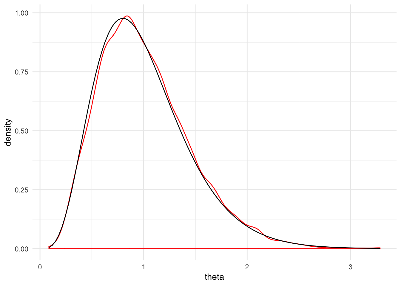
}You can also sample from another distribution. For example, here we’re approximating samples from an gamma distribution. There are also some diagnostic plots that tell us how good the approximation is. The densities match up pretty well.
set.seed(20171124)

theta_sample <- tibble(theta = mh_sampler(dgamma, nreps = 1e4, start = 1, shape = 5, rate = 5))

ggplot(theta_sample, aes(x = theta)) +
  geom_density(color = "red") +
  stat_function(fun = dgamma, args = list(shape = 5, rate = 5)) +
  theme_minimal()